
![]()


Articulation
and the Small Room This paper first presented
at the 85th AES Convention INTRODUCTION The Modulation Transfer Function (MTF) is used in room acoustics as a descriptor of the effectiveness of transmission down the signal path, between the speaker and listener. A major application for this has been speech intelligibility. Basis for MTF analysis is the signal to noise ratio. Noise can be any sound masking effect, steady state noise, transient noise of reverberation or apparent noise due to adjacent octave sound levels. Narrow band MTF is used in the present work.
This is in contrast to the octave band methods common to traditional
speech intelligibility. Here, pure tone modulation used to develop
spectral response detail. A rapidly gated, slow sine sweep is the
test signal for the articulation response curve. This technique
allows blurred transmission bands to be specifically identified.
These narrow ranges of poor articulation are both audible to the
listener and visible in hard copy data. Changes to the room acoustic
are also easily documented. The responsiveness of this test to room
acoustics in addition to the fine grain spectral information in
the articulation response curve suggests that this system be used
as a diagnostic tool. Although originally developed to demonstrate
small room acoustics in the lower registers, it has found use in
the full range of room sizes from the amphitheater and auditorium
right through to recording studio vocal booth. |
| |
| I ARTICULATION RESPONSE CURVE (ARC) A. RATIONALE The Modulation Transfer Function (MTF) is used in room acoustics as the descriptor of effective signal transmission between speaker and listener. A popular application of the MTF is for speech intelligibility. Here we look at an application of MTF developed for precision playback environments such as the hi-end, hi-fi listening room and the recording studio. The suitability of the standard Speech Transmission Index (STI) approach falls short on numerous points in these smaller spaces that have high musical articulation requirements. The spectrum segment useful for STI prediction or measurement starts at the 125 Hz band and each octave band is weighted for significance in speech recognition. Music occupies two octaves lower than the range used for STI work, half the keyboard is below Middle C 2 5 2 . The weighting of these and other octaves in a calculation is not yet established. The musical spectrum and the relative significance of each octave band may well not be the same as for speech. The Music Transmission Index (MTI) may be convertible to STI, but the converse may not be possible. This would be due to the relative lack of full bandwidth information in the STI. Clearly, research remains to be done in this area. The STI joins the group of single index acoustic descriptors, such as NRC, dB, A, IIC, RT60, et. al. Architectural specifications can be satisfied with a single index indicator. Acoustical engineers and consultants engaged in diagnosis and remedy have always required spectral detail and the subject of intelligibility is no different. Measured STI only needs the signal to noise ratio to be detected. Tracking octave band decay rates is one method used and monitoring modulated octave band noise levels is another. Both use selected octave bandwidths and yield a single intelligibility rating. The approach contributes little to the diagnosis of room acoustics. The present technique provides narrow band spectral articulation information. This facilitates diagnostic efforts and evaluation of STC. The predictive side of MTF analysis requires the ability to accurately estimate the signal to noise ratio. The noise level is due to the reflections in the room and due to its reverberation. Predictive methods that use room reverberation decay rates have the prerequisite imposed that the room sound field is instantaneously diffuse and has an exponential decay rate. A non-linear method of predicting noise levels is to use ray tracing of the first 30 reflections. This method better correlates with measured STI. Complex room geometry limits this method. Neither linear acoustics nor ray tracing can be used for predicting in small rooms dominated by room resonant mode decays. The musical line is characterized as a rapid staccato of complex tone bursts. Music then is a set of musical lines, overlaid and intertwining one another. The basic element of this woven fabric of music is the tone burst. The acoustic descriptor that relates to musical articulation may well be the tone burst, indeed a rapid staccato of bursts. Such a signal has been used for harmonic distortion analysis room acoustic transmission path. Here we only desire measurement of the signal envelope and the faithfulness of its modulated transmission. Wave form reproduction, although important, is not the issue addressed. A synthesis of these constraints and requirements
is embodied in the present approach to MTF. The Articulation Frequency
Response Curve (AFC) is a relatively simple, direct physical measurement.
Equally important is the subjective aspect. The auditor in a precision
listening setting can play the test signal over headphones and hear
the rapid, clean staccato of tone bursts whose frequency is slowly
varied. The auditor expects the room acoustic to play this signal
accurately. By removing the headphones and listening to the same
signal in the playback room, defects in the transmission path become
quite audible. In a small room, articulation dramatically varies
with frequency. Typically, there are tenth-octave bands of totally
garbled transmission adjoining similar sized bands of quite intelligible
transmission. The Articulation Response Curve is a fine-grained
quantification of the “fast tracking” ability of a listening
room. |
| II COMPARISON WITH TRADITION
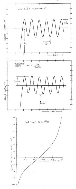
1. Signal Intensity (I)
The mean signal intensity (Io) is modulated by the modulation amplitude (mIo). 2. Modulation Index (m)
It is also expressed in terms of the signal level Is = mIo and the noise level IN = Io - mIo. 3. Modulation Transfer (MT) MT = 20 log m 4. Signal to Noise Ratio (SNR)
It can also be expressed in terms of the modulation index.
|
The offset is 12 dB and the range is 30 dB. 6. Speech Transmission Index (STI)
The weighting factors (WK) normalize to 1.
7. Octave Masking Effect (mO)
The impact of simultaneous independent masking effects is carried by multiplying their independent modulation indices together. m = m1 x m2 |
|
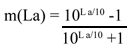
1. Signal Modulation Level (La) 2. Modulation Index m(La)
Upon rearrangement, the modulation index is resolved solely in terms of measured level fluctuation (La).
3. Modulation Transfer (MT)
4. Signal to Noise Ratio (SNR)
5. Transmission Index (TI)
|
6. Mean Transmission Index
(TI) The STI octave band weighting factor (WK) here is undefined. It will be carried in the form of (Wi) to suggest that a listener based preference fit option still remains open. The octave bandwidth weighting actor in STI appears here as a “log frequency” term in the averaged 5.
7. Octave Masking Index (mo) A given mean intensity level is given by the mean sound level (L)
This single level shift is of small consequence but cumulative effects can occur due to a very rough response curve loaded with room resonances. Only 4 such 10 dB shifts would produce a 90% masking index.
|
| III APPLICATIONS A 1. The Burst 2. Duty Cycle The burst has a square wave modulation. Typical MTF bursts are sine wave modulated, either amplitude or level. Here the square wave modulation has ringing in it, visible in both the on and the off parts of the duty cycle. A ramped attack and decay would reduce the ringing effect. Although the pure tone quality of each burst is degraded by the low level ringing, this coloration provided unique cues for the subjective perception of attack transients. At about 2 dB articulation level, the LF ringing loses audibility—this may suggest a method to evaluate perception thresholds of tonal transients.
|
| 5. The Complete Test B. THE RECEIVED SIGNAL 1. The Test Setup 2. Articulation Response Printouts
|
Ramps, both up and down take the place of the sharp attack and decay of the articulate signal. The sustain does not hold flat, it is foreshortened by the ramping transitions. In this inarticulate space, the room mumbles, slurs and often will “double-tongue” the rapidly gated signal. 4. Articulation Response Curve |
| IV ANALOG TRANSMISSION INDEX A. APPROXIMATION TO TI 1. Fitted Curve
2. Circuit Diagram for Measurement If the frequency sweep is a log sweep instead of linear, then log frequency weighting will be maintained by integrating over time. Substantial signal conditioning has been left out of this circuit to retain a sense of propriety integrity but the basic elements are presented.
|
B. DISCUSSION OF La AND Log La 1. Modulation Level (La, dB) It is semantically possible to propose that an effect of negative articulation could exist and not be detected by the present circuit. This occurs whenever sound levels in the dwell period exceed levels, attained during the burst. This seems to be able to happen at a frequency for which sound cancellation occurs. The modulation transfer function is not defined in this situation of negative modulation level. Negative modulation is physically improbable. It takes time for resonant conditions, strong enough to cancel a direct signal, to be developed inside the room. The direct signal will exceed reverb levels during this initial energy buildup period in the room. During this transition period, the direct signal will be heard. Energy is always split between the burst and dwell periods. 2. Articulation Level (10 Log La, dB) This is also measured in dB and the scale is adjusted so that 1.0 dB articulation is equal to zero articulation level (Ref, 1dB). This is really mathematically arbitrary but set here with considerations. The listener’s minimum perceived level change is 0.4 to 0.5 dB for any tone. For the practical purpose of signal burst reproduction 1 dB level differences though audible have little to no perceived value for depicting quality music transition detail. Therefore, it was chosen as zero dB. Regardless, this is an empirical curve fitting arrangement and a different reference here would be reflected in a different DC offset constant than 0.08 above.
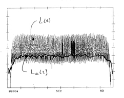
1. Constant Modulation Test Signal Two curves are shown here. The sound L(t) level vs. time articulation response curve is the wide4 fluctuating line. Overlaid on it is a solid, slowly changing and relatively flat line, the Modulation Level, La(t). 2. Upper Limits to Sound Level 3. Calibration
1. Modulated Sweep Response Curve The overlaid solid line is the transmission index vs. frequency at the 8 Hz gated modulation rate. The mean TI would be the averaged value of this curve. 2. This curve is a linear frequency sweep and the mean TI requires log frequency weighting. If a log frequency sweep was used instead of linear, then straight integration of the TI in time would produce the mean TI. Linear sweep is often used in low frequency
room measurements. It is said the ear hears quasi-linear frequency
scale below 200 Hz. The log sweep spends ¾ of the time below
170 Hz about ¼ of the frequency range to be explored. The
remainder ¼ test time packs the remaining ¾ frequency
range (200 to 800 Hz). Although log frequency sweep accommodates
a simple integration scheme for the mean TI, it most likely is not
sampling sufficiently the room articulation. A more sophisticated
integration must be used. |
| V
SAMPLE TESTS
A. ROOM SEQUENCE A listening room, 8’ x 14’ x 18’ with double sheetrocked walls and concrete floor is tested at various stages of acoustic treatment. Fundamental, is the use of corner-loaded bass traps. The mic is placed at the hi-fi listener’s position and two speakers, in phase are located at the opposite end of the room in a stereo setup.
2. Absorption Added in Stages a. Here, a simple Tx6 set has been added to the front of the room behind the speakers. Already a substantial pattern of low level articulation is established throughout the entire test. The hills and valleys have grown less severe and are covered better with a wider articulation band. Note also the overall flatness, the room is being acoustically EQ’d. b. The next setup adds traps (16x3 plus 11x3 pair stacks) at the back of the room. Again, the frequency bands of improved articulation widen. The severity of the peaks and valleys is more reduced. A few peak/valley patterns have even disappeared. The softening of the peak/valley profiles means the “Q” of the room, the sharpness of its resonance responses, have been lowered. As the room resonances are damped, the peaks drop, the valleys rise and there is an overall softening effect to the room response curve.
|
|
d. The head wall traps are the next to be set, 6-11x5 ½ Rounds plus a single column of 11x6 Full rounds in the center. This develops stage depth, clarity and imaging detail. Dramatic articulation improvement is seen broadband, the peak/valley terrain flattens substantially. The width of the articulation patterns have grown quite wide and improvement is seen in the mid-bass. The front/rear energy storage system of the room has been dampened to make this marked improvement. e. Finally we have added the rear wall. A 16x3 + 11x5 center column and 4 sets of 11x5 ½ Rounds with one more pair on the front wall. The result is a very wide and steady articulation pattern that extends even into the deepest bass. Peaks and valleys now even more are soft, rounded. The room still retains a strong, comfortable ambience. If you compare the overall before and after room articulation signatures, you will see that the sound levels below 100 Hz have not changed and those above 100 Hz are depressed by about 5 dB. In addition, we see that below 400 cycles the articulation signature increases from 2 to 8 dB and above 400 from 10 to 18 dB.
|
|
4. Full Acoustics Plus Equalizer a. The “full on” room has also been tested. This is not too unlike the typical dedicated Hi-end reference listening room. Basically, a carpet has been added along with floor bounce traps. All the traps of the prior setup (#6) have been elongated from their 5-foot height to a full floor to ceiling length. A major articulation improvement is noted, especially in the 20 to 400 Hz range. The natural acoustic #Q is taking a strong control, the low-end boom below 100 is almost gone. b. Finally, to this “ultra” system, we degrade its sonics but add equalizer effects. Again the EQ is set with pink noise, RTA and 1/3 octave equalizer. The result is pretty flat, and articulate response. There are a few small band widths with poor articulation remaining. Even these may well be cleaned up with additional tweaking. Again the ringing effect of the equalizer is clearly audible in this test, something undesired in precision audition.
|
|
1. RTA and Room Treatment Sequence Relatively minor corrections towards flattening the spectrum sound levels with no loss of deep bass sound power is how RTA sees the effects of the full on acoustics. Clearly RTA doesn’t begin to suggest the fast tracking ability of the listening room. 2. RTA and Slow Sine Sweep The RTA levels are weighted higher with increasing frequency. This is due to wider bandwidths, more 1 Hz levels being added together. The equivalent narrow band spectrum can be had by subtracting the bandwidth weighting term from each bandwidth level. L = 10log f + 10log 23% The 1/3 octave has 23% bandwidth. When the two curves are overlaid the general tendency is seen but the detailed narrow band sweep cannot be even inferred by the 1/3 octave measurement. |
|
For example, 1/3 octave EQ suggests that the 250 Hz band should be cut some 5 dB. However, the articulated sweep response shows that the problem high sound level is a 1/3 octave band centered at 180 Hz. C. SLOW SINE AND MODULATED SWEEPS Here we compare the slow sine sweep to the modulated sweep. The sound levels at the listener’s position are recorded in both cases between 20 and 800 Hz.
|
a) Articulation levels La of 12 to 15 dB attain peak sound levels equal to that of the slow sine sweep levels. b) Articulation levels that are less than 12 dB fall short of the slow sine sweep level by an amount approximately equal to: 15 - La. c) Strong articulation is associated with wide bandwidths of relatively uniform sound level on the slow sine sweep response curve. d) The lower the “Q” of sine sweep response curve the stronger the articulation signal. e) Very low articulation levels are always accompanied by a very sharp, high “Q” room resonance section of the room response curve. f) Rapid sound level changes in the slow sine sweep curve mark frequency bands with poor articulation response. |
C. ROOM MODES AND “Q” From the above it is clear that room mode spacing and the adjustment of room resonance “Q” are controlling variables in the development of articulation response in small rooms.
2. Modulation Level La and Room
“Q” Q x La = 180 Since the minimum La for acceptable listening is about 5 dB, the most probable maximum acceptable “Q” will be about 36. For the very desirable La of 10 dB we have room resonance “Q” of 18. The “Q” of a typical room is often 40 to 50 prior to specific acoustic conditioning. |
D. LINEAR “Q” VS La The classic sabine equation uses diffuse exponent sound fields. The “Q” vs. La relationship can be predicted, it is seen to not fit the measured relationship. This is expected because the sound field in small rooms and lower octaves does not exponentially decay.
The frequency of the resonance (f) part of the dependant variables. Q = 1/22 RT60
The gated tone burst has burst rate (F) and its dwell period is the time allowed for sound level decay.
An 8 Hz gated frequency yields an equation relevant to the present test.
3. Linear “Q” and La
For linear decay the Cis directly proportional to frequency. This is not what is measured, a constant. Since both definitions used, “Q” and La assume a linear acoustic relationship with RT60, neither can be identified as the non linear term at this point. |
| DISCUSSION The goal of this project has been to explore the Transmission Index of small rooms in the lower octaves. The rapidly gated slow sine sweep is an effective test signal. Although envelope shaping of the attack and decay should be explored, the existing coloration led to the observation that low level coloration becomes inaudible at a higher modulation level than does the modulation itself. This suggests that “quality” detection thresholds may well be much different from “quantity” detection. Research in perception along the lines of complex signal detection thresholds needs to be applied to the present work. The difference between the linear and measured QLa term stands to illustrate that the prediction of TI in the lower octaves in small rooms has yet to be accomplished. More empirical work also needs to be done in this area. The observation presented here is only based on one data run. A new, complex test signal and detection method may be considered to directly measure the masked partial signal level. A correlation between pure tone modulation levels at the partially frequency and the masking level of the partial wherein a complex tone burst ie. Linear, additive effects, may be fruitful. The TI equation has been approximated here by a fitted curve using the same single variable. The only reason for this is to access the convenience of a relatively simple analog circuit. Further work with the exact equation ought to be completed using analog or computational methods to develop the TI. There also may be additional terms added to reduce the error of the approximation curve. There lies ahead a great opportunity to work on the theoretical side of the Transmission Index at lower frequencies in small rooms. The first step aside from large halls in linear acoustics was the ray tracing method, but this is not applicable to small room resonant modes. The relative level effect needs to be factored into the present TI approach. A room with strong level changes in a slow sine sweep must be penalized when compared to a room with a relatively flat response. A method to isolate this effect needs to be developed and produce an independent modulation index. In general, standards for speech in small
rooms need to be applied to this work. The performance of STI analyzers
needs to be compared to traditional listening tests in small classrooms
where modes exist in the speech range. In large halls, little emphasis
is given to the lower speech octave, 125 Hz. Small rooms, with their
room modes and typical lack of low frequency absorption, may well
require re-assessment of this weighting. |
| CONCLUSION A method that develops spectral response curves for articulation has been demonstrated. The measure variables have been written into the equations that define the Modulation Transfer Function and the corresponding Transmission Index. The signal to reverberant noise level is directly measured and there is no conversion of data that requires the assumption of linear acoustics. The equipment used to make this test is relatively common. The source is a pre-recorded cassette test signal. Analysis will use as little as a sound meter and strip chart recorder. By adding a circuit for signal processing, the Transmission Index response curve can be developed. With additional circuits even the STI can be stated. The STI is fast becoming a standard specification.
Engineers and consultants require a spectral version of the Transmission
Index in order to remedy the acoustics. Now that this simple and
low cost articulation test method has been shown to produce detailed
spectral information, it is hoped that this technique will be the
forerunner of a new class of sound system analysis. |
BIBLIOGRAPHY (The following were used in the preparation of the paper) Houtgast, T. and Steeneken, H.J.M., Predicting Speech Intelligibility in Rooms from the Modulation Transfer Function Parts I, and II. ACUSTICA VOL 46, 1980. Houtgast, T. and Steeneken, H.J.M., A Review of the MTF Concept in Room Acoustics and Its Use for Estimating Speech Intelligibility in Auditoria. JASA 77 (3) March 1985. Schroeder, M.R., Modulation Transfer Functions: Definition and Measurement. ACUSTICA Vol 49 (1981) 179. Houtgast, T. and Steeneken, H.J.M., A Physical Method for Measuring Speech-transmission Quality. JASA 67 (1) Jan 1980. Houtgast, T. and Steeneken, H.J.M., The Modulation Transfer Function in Room Acoustics as a Prediction of Speech Intelligibility. ACUSTICA Vol 28, 1973. Kryter, Karl., Methods for the Calculation and Use of the Articulation Index. JASA 34 (II) Nov 1962. Polack, J.D., Alrutz, H. and Schroeder, M.R., The Modulation Transfer Function of Music Signals and its Application to Reverberation Measurements. ACUSTICA 54 (1984). Demany, L. and Semal, C., Amplitude and Frequency Modulation. ACUSTICA 61 (1986). Fastl, H. and Hesse, A., Frequency Discrimination
for Pure Tones at Short Durations. ACUSTICA 56 (1984). |
 A.
DEFINITION OF STANDARD TERMS
A.
DEFINITION OF STANDARD TERMS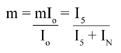

 5.
Transmission Index (TI)
5.
Transmission Index (TI)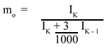
 B.
MTF IN PRESENTLY MEASURED TERMS
B.
MTF IN PRESENTLY MEASURED TERMS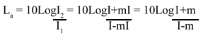


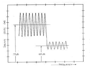 Assume,
for example, equal octave fraction band widths for a low frequency
75 dB level followed by a weaker 65 dB level
Assume,
for example, equal octave fraction band widths for a low frequency
75 dB level followed by a weaker 65 dB level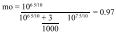
 .
THE TEST SIGNAL
.
THE TEST SIGNAL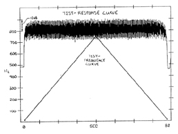 3.
Frequency Range
3.
Frequency Range 4.
Signal Intensity
4.
Signal Intensity 3.
Burst Sequence
3.
Burst Sequence The
key is the TI term. Within the range of desired values a simple
expression has been found to closely match within a few percent.
Also note the expression is in terms of La, the presently
measured modulation variable.
The
key is the TI term. Within the range of desired values a simple
expression has been found to closely match within a few percent.
Also note the expression is in terms of La, the presently
measured modulation variable.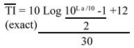

 C.
L, La AND Log La OF TEST SIGNAL
C.
L, La AND Log La OF TEST SIGNAL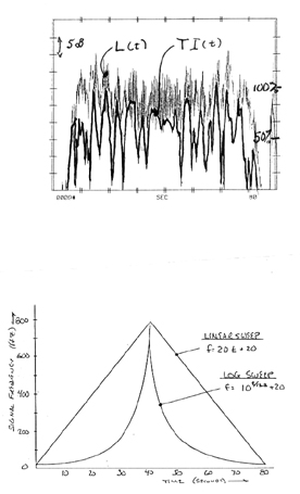 D.
L, La AND Log La OF RECEIVED SIGNAL
D.
L, La AND Log La OF RECEIVED SIGNAL 1.
Bare Room Response
1.
Bare Room Response c.
Next is added a side wall treatment, 4 sets of 9” x 5’
½ Rounds. This controls stage width and imaging, lateral
flutter and cross talk. It develops overall a much deeper articulation.
It produces wide bands of continuously full articulation, some 200
Hz wide between 400 and 600 Hz. Yet, curiously there seems to be
some areas of thinning, reduced articulation around 150 Hz.
c.
Next is added a side wall treatment, 4 sets of 9” x 5’
½ Rounds. This controls stage width and imaging, lateral
flutter and cross talk. It develops overall a much deeper articulation.
It produces wide bands of continuously full articulation, some 200
Hz wide between 400 and 600 Hz. Yet, curiously there seems to be
some areas of thinning, reduced articulation around 150 Hz.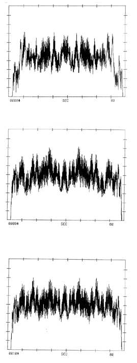 3.
Equalizer Added
3.
Equalizer Added B.
1/3 OCTAVE PINK NOISE, RTA
B.
1/3 OCTAVE PINK NOISE, RTA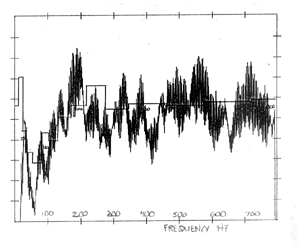 3.
RTA and Articulated Sweep
3.
RTA and Articulated Sweep
 1.
Observations and Tendencies
1.
Observations and Tendencies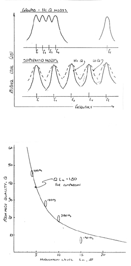 1.
Mode Spacing
1.
Mode Spacing 2.
La and RT60
2.
La and RT60